Summary
The GRate project work to reconstruct the Greenland Ice Sheet (GrIS) Margin through the Holocene will leverage several different methods, including both those used in the Snow on Ice project, and those that are new for this phase.
A method that contributed to our understanding in SW Greenland In the Snow on Ice project, was the radiocarbon dating of sediment samples cored from pro-glacial lakes. The lakes are created as the ice sheet melts and shrinks in size, leaving behind depressions along the ice edge that fill with glacial meltwater. Sediment collected from these lakes were used to track ice sheet retreat and expansion. While this method was an important part of our work in SW Greenland for the Snow on Ice Project, other methods like exposure dating and reconstructing relative sea level will take priority in the GRate project expansion to the rest of the ice sheet.
A second important tool used in Snow on Ice was exposure dating, or the sampling of quartz in rock for cosmogenic nuclides. Dating glacial deposits is a technique used to establish past extent of the ice sheet, and determine rates of ice sheet recession. In Snow on Ice we were able to date these glacial deposits in moraines, rows of accumulated rock and rubble deposited on the landscape as evidence of areas where the ice sheet stalled for a period of time as it retreated inland. Exposure dating these moraines, along with free standing glacial erratics (large rocks left behind on the landscape by the ice sheet as it retreated) provided a timing for the ice retreat from the SW region of Greenland. We will adjust our approach for this next phase of work, in both what is sampled, and the technique used, shifting fom Beryllium-10 (10Be) to Carbon-14 (14C) exposure dating. Jason P. Briner, University at Buffalo, PI, Nicolás Young, LDEO, PI, and Joerg Schaefer, LDEO, PI, will lead the work for this part of the project.
An additional tool that will be part of GRate is the construction of relative sea level (RSL) curves in areas where the data is either absent or not well constrained. Karlee Prince, student at University at Buffalo, Jason P. Briner, University at Buffalo, PI, Lambert Caron, JPL, are leading the RSL “data-model” comparison, along with collaborator Ole Bennike, GEUS.
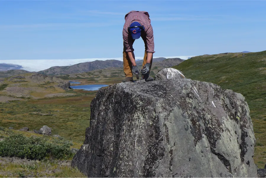
Image: Nicolás Young collects a rock sample for exposure dating from a large glacial erratic dropped in southwest Greenland by the ice sheet as it moved across the landscape. This technique was highly effective for the Snow on Ice project in SW Greenland. In the GRate project we will continue to rely on glacial erratics as well as bedrock samples.
14C Exposure Dating
The GRate project will build on both the Snow on Ice work and other studies, where areas with robust chronology reveal that the GrIS retreated off the continental shelf and onto land approximately 12 ka ago, near the beginning of the Holocene. Exposure dating can include a range of different isotopes (14C, 10Be, 26Al and 36Cl) all of which can be used to reconstruct the history of the ice sheet margin over the past 20,000 years. With different half-lives, each has a best use in a specific location and set of conditions. For this project 14C has been selected as the best tool for several reasons explained below.
In Snow on Ice 10Be was the primary isotope used in cosmogenic dating for the project. While it does not occur naturally in quartz, once the quartz is touched by cosmic rays 10Be becomes trapped in the crystal lattice of the quartz, beginning its slow accumulation and providing an exposure time clock. One of the important features of using cosmic ray exposure as a dating technique is that the rays do not penetrate extremely deep into the rock, so isotopes only accumulate near the top. Therefore, rock surfaces that have had previous exposure to cosmic rays can still be dated, but only if there has been glacial erosion at amounts that will remove any residual isotopes in the surface of the rock (called inheritance). In SW Greenland there has been sufficient bed erosion from the ice during the last ice age to remove concerns of inheritance. This means the exposure ages from SW Greenland can faithfully record the last time the ice left and began a new clock (the timeperiod of the Holocene).
In many areas of Greenland rock samples are plagued by inheritance, as previous cosmic ray exposure that has not been glacially erroded away through time. With the long half life of 10Be (t1/2 = 1.39 × 10⁶ years), areas with minimally erosive environments, such as in E and N Greenland, will require a different technique. In-situ 14C dating has a relatively short half-life (t1/2 = 5700 years), allowing previously accumulated in-situ 14C to decay to undetectable levels after ~30,000 years of ice burial. Previous work by N. Young and others has shown in-situ 14C to be effective in capturing ice retreat ages in NW Greenland, where 10Be ages had been plagued by inheritence.
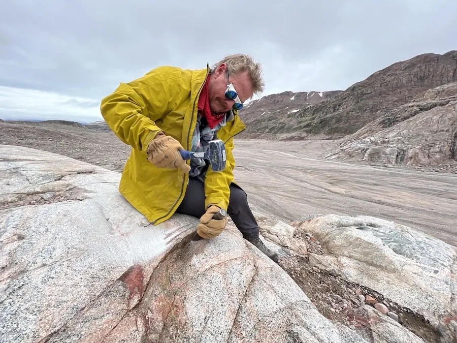
Image: Joerg Schaefer collects a rock sample for exposure dating in E Greenland.
Additionally, in Snow on Ice, the work focused on samples from a series of glacial moraines, a prominent feature of SW Greenland left there by the retreating ice sheet. However, moraine series are not present in the areas of Greenland we target in GRate. In E and N Greenland, we will rely on boulder fields and bedrock for cosmogenic exposure dating. For both these reasons the GRate project will be using a different approach than in Snow on Ice.
For GRate four regions in N and E Greenland will be targeted for generating chronologies of ice retreat. The work will constrain two critical ice-margin benchmarks needed for our Greenland-wide modeling effort: the timing of 1) ice-margin retreat out of the ocean and onto land following the last deglaciation, and 2) ice-margin retreat to (and likely behind) its present margin in the Holocene.
Relative Sea Level History
Relative Sea Level (RSL) refers to how the ocean height rises, or falls, relative to the land/shore at a given location. RSL reconstructions (tracking them through geologic history) are important tools for understanding the effects of the weight (or load) of the ice directly next to the ice sheet, and how, and over what period of time, that loading and unloading takes place. This is also called 'near-field' ice loading signals. Areas that are directly adjacent to the ice sheet, are highly affected by isostatic effects. The GRate team will will produce new RSL and ice-margin histories in key areas around Greenland to help fill important data gaps in spatial coverage. A key piece of this will be to generate RSL curves in two key sites that will help to plug holes in spatial coverage of RSL data (see figure below).
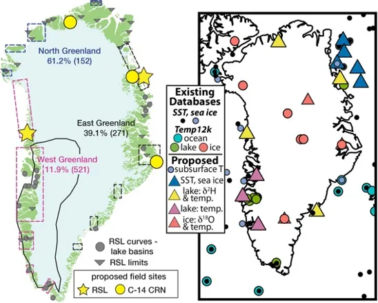
Figure: The insostatic response of the area to the loading and unloading of the ice is developed through reconstructions that can help to constrain ice sheet history. There are limited data available for large portions of Greenland’s perimeter. Grate proposes to add RSL data by collecting field data in areas shown by the yellow stars on the image to the left and then adding that data to existing geochronolgy and RSL data to improve our models.
Site # 1) In NW Greenland there is no RSL data of any kind between Qeqertarsuup tunua (Disko Bugt) at the southern end and Thule in the northern end. This extensive section of Greenland’s perimeter spans ~1000 km of coastline. We will develop a RSL curve near Upernavik in Qimusseriarsuaq (Melville Bugt) NW Greenland. This area of the ice sheet margin is marine dominated with deep fjords extending from ~50 to >100 km inland of the present ice margin. This means there is high potential for significant inland retreat in this part of Greenland, both during the middle Holocene and in the future. Focusing on this area for signs of retreat and re-advancement could reveal ice margin sensitivity to forcing by Holocene climate.
SIte #2) In Germania Land, NE Greenland, there is effectively a ~500 km gap in RSL data coverage between the Kejser Franz Joseph Fjord area to the outlet of the Northeast Greenland Ice Stream. This area is largely ice free.In both sites, we will use the isolation-basin method in this location. This method tracks how the crust rebounds after ice is unloaded during deglaciation and brings land up and out of the ocean. To reconstruct sea level, we collect and analyze sediments from a series of basins that were isolated from the ocean during different stages of ice sheet history (see figure below).
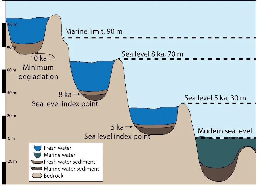
Caption: Image showing a series of isolated basins that formed in a tiered set up as the ice sheet retreated through time. The highest elevation basin would have been created first, with each subsequent basin created as sea level fell throughout time. (Image by K. Prince)
In both sites location there are a stair-case of lakes, in close proximity to each other, and yet at differing elevations. Within each basin there are three phases of of sedimentation critical in establishing RSL fall or in establishing ice sheet readvancement: 1) full marine phase; 2) a brackish or mixed salinity phase; 3) a freshwater phase. Samples will be collected for stratigraphic and micro- and macro-palaeontologic analysis (for ease of identifying freshwater/marine sediment contacts) and radiocarbon dating.
An additional piece of our RSL reconstruction will involve combining newly developed datasets with syntheses of all available geochronology and RSL data to do a systematic data-model comparison.
GRate is funded under the National Science Foundation (NSF) Office of Polar Programs.